Skip to content

Solving SVP in Dimension 2 ​

Reduced Basis ​

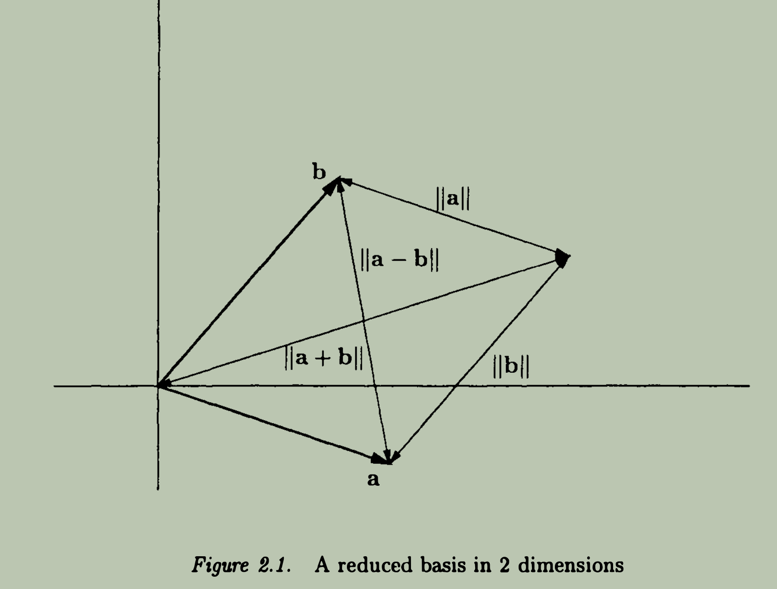
Definition 2.1 - Let [a,b] be a lattice basis. The basis is reduced if

|∥a∥,∥b∥≤∥a+b∥,∥a−b∥

Intuition Behind

Consider constructing a triangle with known two edges a and b, the third edge is unknown. If [a,b] is reduced, by definition, we can say that a,b are the shortest two edges of the triangle.


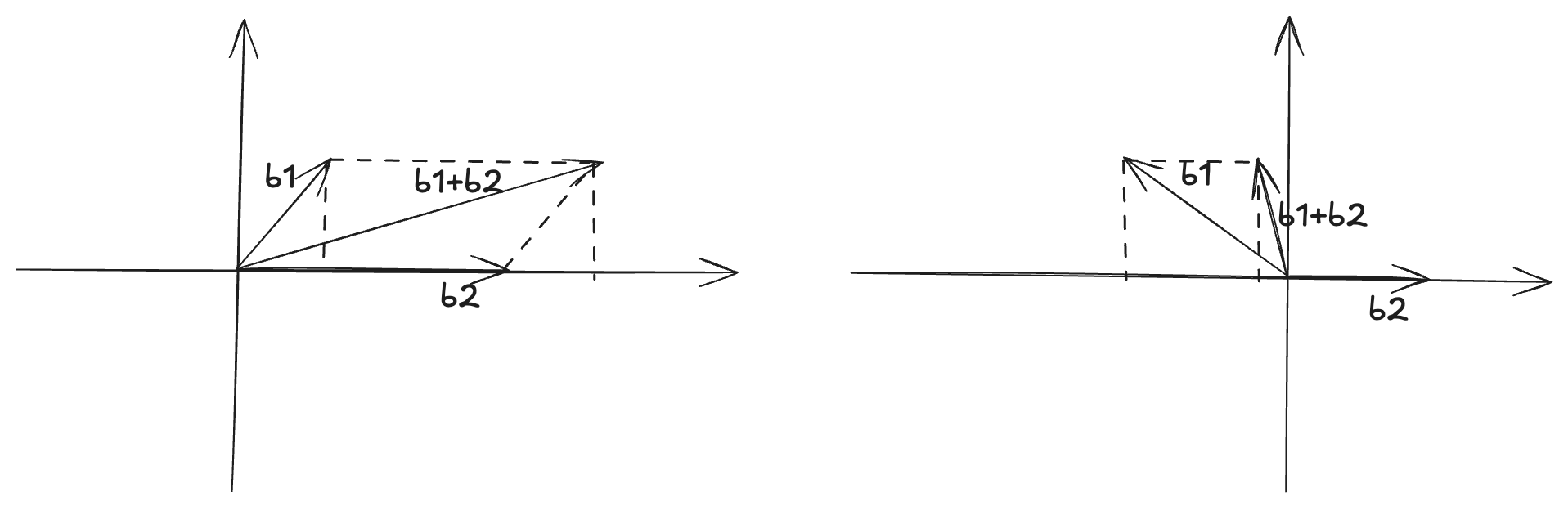
Lemma 2.1 - Consider three vectors on a line, x,x+y,x+ay, where a∈R. Then if ∥x∥≤∥x+y∥ then ∥x+y∥≤∥x+ay∥, moreover ∥x+y∥≤∥x+ay∥.
Reduced Basis 1

Explanation

Intutively, given x,x+y, if ∥x∥≤∥x+y∥, then we are clear that both x and y are pointing in roughly the same direction, and adding any multiple of y to x+y will only increase the norm.

Similarly, if ∥x∥≤∥y−x∥, then y and x are pointing in roughly the contradictory direction, furthermore, ∥x∥≤∥y−x∥≤∥ay−x∥.


IMPORTANT

So what is the relationship between reduced basis and the successive minima of the lattice?

Theorem 2.2 - Let [a,b] be a lattice basis, and let λ1 and λ2 be the successive minima of the lattice. If the basis is reduced, then ∥a∥=λ1 and ∥b∥=λ2.
Reduced Basis 2

Explanation

From the definition of reduced basis, we know that whether a and b have the same direction or not, we need to ensure that either of a or b is the shortest vector in the lattice. Without loss of generality, we assume ∥a∥≤∥b∥ :

  • if a,b have the same direction, then ∥b∥≤∥a+b∥.
  • if a,b have the opposite direction, then ∥b∥≤∥a−b∥. put them together, we need to ensure ∥b∥≤min{∥a+b∥,∥a−b∥}. Therefore,
∥a∥≤∥b∥≤min{∥a+b∥,∥a−b∥}

In general, we have

∥a∥,∥b∥≤∥a+b∥,∥a−b∥

namely, basis [a,b] is reduced.


Gauss Algorithm ​

Definition 2.2 - For a lattice basis [a,b], without loss of generality, we assume ∥a∥≤∥b∥, if ∥a∥≤∥a−b∥≤∥b∥, then we call the basis [a,b] a well-ordered basis.


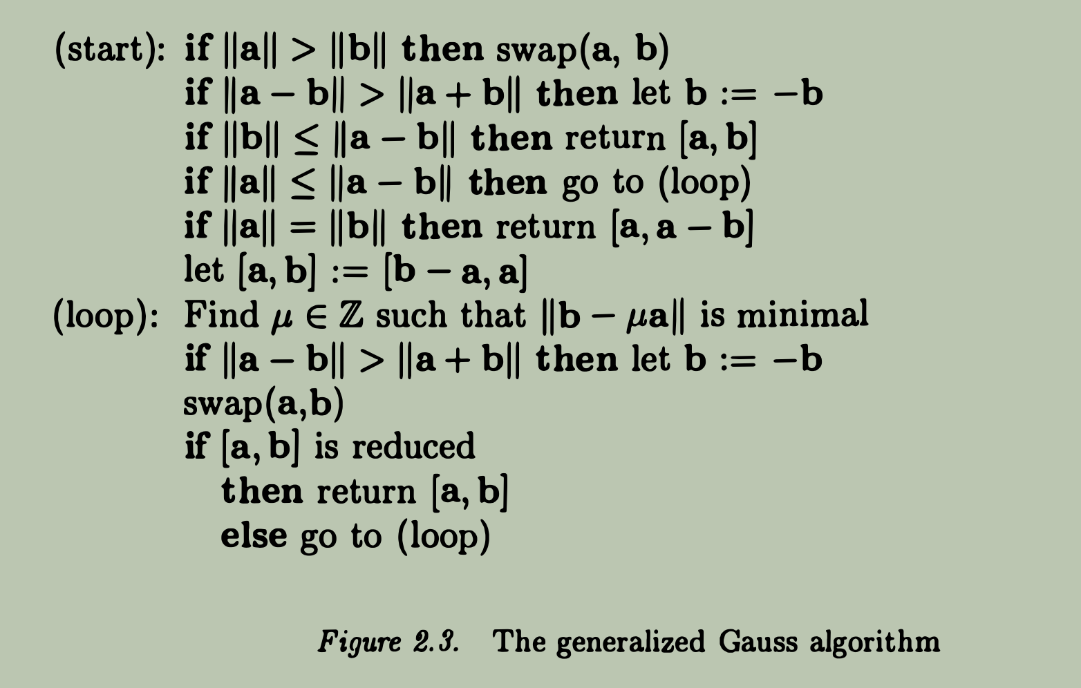
Algorithm

Gauss Algorithm

Explanation

For the line-1 and line-2, we are trying to ensure

  • lattice vector a is the smaller one, i.e., ∥a∥≤∥b∥
  • both lattice vectors a and b are in the same direction, i.e., ∥a−b∥≤∥a+b∥.

After then we will consider following cases :

  1. For the line-3, it is the simplest case where ∥b∥≤min{∥a+b∥,∥a−b∥}=∥a−b∥, in this case, we must have :

    |∥a∥≤∥b∥≤∥a−b∥≤∥a+b∥

    then the basis [a,b] is strictly reduced, and they are in the same direction, return [a,b].

  2. For the rest of lines, it is the case of ∥a−b∥<∥b∥, there are two subcases to consider:

    • (2.1) for the line-4, ∥a∥≤∥a−b∥<∥b∥, then basis [a,b] is a typical well-ordered basis, and they are in the same direction.

    • (2.2) for line-5 and line-6, ∥a−b∥≤∥a∥≤∥b∥, then there are two subcases to consider :

      • (2.2.1) for the line-5, ∥a−b∥≤∥a∥=∥b∥, this is a very special case, ∥a∥=∥b∥ and ∥a−b∥≤∥a∥ ensure that vectors a−b and a are in the same direction, in this case, ∥a∥=∥b∥≤∥2a−b∥. Since ∥(a−b)−a∥=∥b∥, thus the basis [a−b,a] is reduced, and they are in the same direction, return [a−b,a].

      • (2.2.2) from line-6, ∥a−b∥≤∥a∥<∥b∥, we do not know the whether a−b and a are in the same direction or not, but ∥a∥≤∥b∥ and ∥a−b∥≤∥a∥ ensures that vectors b−a and a are in the same direction, so ∥b−a∥≤∥(b−a)−a∥≤∥a∥. Therefore, the basis [b−a,a] is well-ordered basis.


The remaining problem is how to find the reduced basis through well-ordered basis in the loop :

  1. Since [a,b] is a well-ordered basis, there are other lattice vectors that can be fit between [∥a∥,∥b∥], what we need to do is finding the smallest one. This is achieved by find the integer μ such that ∥b−μa∥ is minimal, then replace b with b−μa.

  2. Now we can check that if the updated basis [a,b] is reduced, but before checking we need to make sure that ∥a∥≤∥b∥, if not, swap a and b.

  3. repeat the above steps until the basis [a,b] is reduced.


Next, we will focus on how to find the minimal vector between two well-ordered basis vectors in the Gauss loop.

Minimal Vector in Gauss Loop

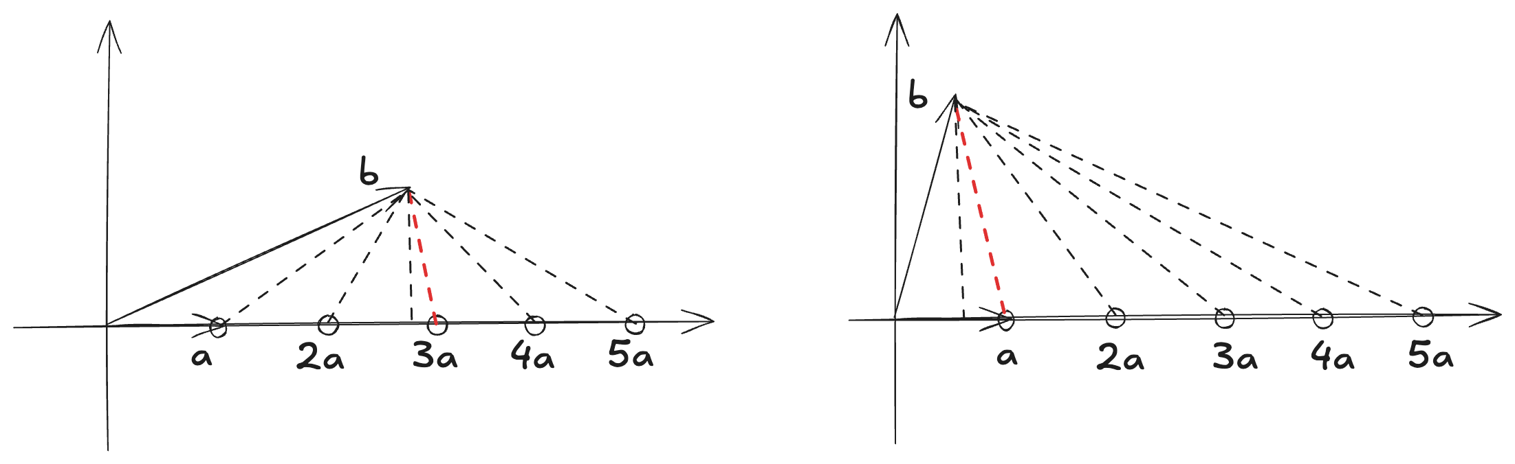
Lemma 2.3 - Let a,b be two vectors such that ∥b−a∥<∥b∥. Then, one can efficiently find an integer μ such that ∥b−μa∥ is minimal. Moreover, μ satisfies 1≤μ≤⌈2∥b∥∥a∥⌉.
Gauss Algorithm 1

Explanation

Note that, in Gauss algorithm, before entering the loop, we have ensured that the basis [a,b] is well-ordered, i.e., ∥a∥≤∥b∥ and ∥a∥≤∥a−b∥≤∥b∥. But, this theorem does only mentioned last-half condition of well-ordered basis, i.e., ∥a−b∥≤∥b∥. So this is a more general setting than the well-ordered basis condition.


For better understanding Gauss algorithm, we will specially consider the l2 norm, and explain why we are able to find the minimal vector between a and b in Gauss loop if [a,b] is well-ordered with geometric intuition.

Condition ∥a∥≤∥a−b∥<∥b∥ implies :

  • vectors a,b are in the same direction.
  • projection scalar of b onto a, i.e., ⟨a,b⟩∥a∥2>1/2.
  • the minimal distance between b and a is ∥b−⟨a,b⟩∥a∥2a∥.

Two cases involved in finding the optimal integer μ are:

  1. If 12<⟨a,b⟩∥a∥2≤1, then ∥b−μa∥,u∈N increases as μ moves away from the minimal value ⟨a,b⟩∥a∥2. In this case, μ=1 is the optimal integer choice.
  2. If ⟨a,b⟩∥a∥2>1, then ∥b−μa∥,u∈N increases in the range [1,⟨a,b⟩∥a∥2), and decreases in the range (⟨a,b⟩∥a∥2,∞). In this case, the optimal integer choice must come from either ⌊⟨a,b⟩∥a∥2⌋ or ⌈⟨a,b⟩∥a∥2⌉.

Additionally, we will simply explain why ⟨a,b⟩∥a∥2>1/2 in the contex of well-ordered basis with one diagraph below.
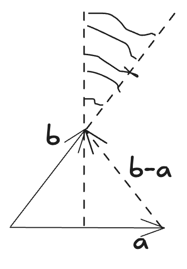
Well Ordered Basis


Why Gauss Loop Works

For now, we have only illustrated how Gauss loop works, and more specially how to find the minimal vector between two well-ordered basis vectors in the Gauss loop. But we have not touched why the loop works? or why we are able to eventually reach a reduced basis through repeated iterations from a well-ordered basis.


We know that the first step of Gauss loop is to find the minimal vector between the two basis vectors a and b which are well-ordered, i.e., b′=b−μa, where μ is the integer that minimizes ∥b−μa∥. Theoretically, the new vector b′ could be :

  1. ∥a∥≤∥b′∥,
  2. ∥b′∥<∥a∥.

For the condition (1), since ∥b′∥=∥b−μa∥ is minimized, so :

  • ∥b−μa∥≤∥b−(μ−1)a∥ implies ∥b′∥≤∥b′+a∥
  • ∥b−μa∥≤∥b−(μ+1)a∥ implies ∥b′∥≤∥b′−a∥

Thus, if ∥a∥≤∥b′∥, then basis [a,b′] is already reduced. The Gauss loop will terminate for this pair of vectors.

For the condition (2), we know that step two of Gauss loop ensures that b′ and a are in the same direction by flipping the sign of the new vector b′ if necessary, i.e., ∥b′−a∥≤∥b′+a∥. Since ∥b′∥<∥a∥, we have ∥b′−a∥≤∥a∥, furthermore, ∥b′∥≤∥b′−a∥≤∥a∥. Therefore, basis [b′,a] is well-ordered.

Then the Gauss loop will continue with the new well-ordered basis [b′,a], repeating the process until a reduced basis is obtained.


Running Time Analysis ​

By analysing the Gauss loop, we know that given input well-ordered basis [b,c], we can obtain a new well-ordered basis [a,b] unless the basis is already reduced. Note that, in one iteration vector b not changed, only vector a is invented. Then repeating the process more times will eventually lead to a reduced basis. So our concern is : is the number of iterations (time complexity) bounded by a polynomial of the input size N (bits of one vector entry)? The answer is yes, but before our final conclusion, a lemma is needed.


Suppose the first input basis vector is [an−1,an], next input is [an−2,an−1], ..., till the last input is [a1,a2], and [a1,a2] is reduced.

Lemma 2.4 - For i≥3, ∥ai∥≤1/2∥ai+1∥.

Explanation

Let [a,b,c]=[ai−1,ai,ai+1], given input well-ordered basis [b,c] output another well-ordered basis [a,b]. Then we need to show the input lengths satisfy ∥b∥≤1/2∥c∥.

As we know, a=±(c−μb) for some integer μ that minimizes ∥a∥. We can consider it with following cases :

  1. μ=1
  2. μ=2
  3. 2≤μ

We omit the details proof here.


Given the input basis [a,b] of Gauss algorithm, and [ak,ak+1] is the first well-ordered basis entering the Gauss loop, after k iterations, we obtain the following inequality :

2k−2≤2k−2∥a3∥≤∥ak+1∥≤∥a∥+∥b∥

Since before entering the Gauss loop, we may have swapping, negation, or substrating operations, but :

∥ak+1∥≤∥a∥+∥b∥

always holds. It is clear that the number of iterations is bounded :

k≤log2⁡(∥a∥+∥b∥)+2

If the number of bits of one vector entry is N, suppose there are m entries in one vector, then :

∥a∥≤m⋅(2N⋅2N)=m⋅2N

So we have :

k≤(N+3)+log2⁡m

As m is fixed, the term log2⁡m is constant, so k=O(N).


Approximating SVP in Dimension n ​


Approximating CVP in Dimension n ​


Published with GitHub Pages.